Model Uncertainty Without Priors (Part 2)

In Part 1 of this post, I described why and how to find parametric models that describe real-world phenomena, and ended with a question: once you have a model, how certain are you that your parameter estimate is the right one? In this post, I’ll introduce an informal notion of uncertainty and describe how to quantify it using martingales, without a Bayesian prior.

---

As a reminder: is a function with inputs and outputs , is the set of unknown parameters that depends on to produce , and together make up what I’ve been calling a model. is the data we’ve collected, i.e., the observed input/output pairs .

Parameter uncertainty §

In this post, my notion of uncertainty is captured by the following criterion: “I am certain of my estimate of if observing slightly different data would not change my estimate of .” Another way of expressing what I mean is: “I am uncertain if slight differences in the data I collected would have resulted in a completely different estimate of .” I intentionally avoid a formal definition of uncertainty because 1) it would require a lot more mathematical/philosophical machinery which is out of scope for this post, and 2) as we will see later, this informal notion of uncertainty is sufficient for some very interesting results.

I’ve been interested in uncertainty for a long time (here are a bunch of posts and a paper). But in this post I’m going to focus on a method I recently learned about that uses martingales (I’ll define this shortly) to make uncertainty quantification of models a lot easier.

Quantifying uncertainty as a Bayesian §

One way of quantifying parameter uncertainty is through the framework of Bayesian probability. Under this framework, uncertainty over parameters is expressed by a probability distribution , which represents the following question: “As a number between 0 and 1, how likely do I think it is that the I picked is the correct one?” By “correct” I mean the true value of that generated the data (assuming your chosen function matches how reality actually works). I will refer to probability distributions as the “belief”, and as the prior belief or simply prior.

When we quantify the uncertainty of our estimate of , we are obtaining a new belief for , given the observed input/output data , i.e., . is also known as the posterior belief. This probability distribution is obtained using Bayes’ rule:

where is the likelihood belief, which essentially answers the following question: “Given parameters , how likely am I to observe the data ?” Assuming the data points are independent given , the likelihood factors as a product of the conditional likelihood of each data point:

The likelihood belief captures any randomness in your function . For example, if your function is

where and is zero-mean Gaussian noise, then the likelihood of a single data point is given by

For the purposes of this post, you can think of Bayes’ rule as a black box that takes in your prior belief , the data , and a likelihood , and spits out a posterior belief :

For example, let’s say the unknown parameter is the outside temperature today. It’s summer, so you believe with 90% certainty that it will be hot, i.e., . Then you look at the weather app on your phone. This is the data : the weather app says it’s cold. Then, assuming you can nicely compute all probabilities involved, you can use Bayes’ rule to get a new belief for what you think the actual temperature is outside, e.g., .

Here’s the big issue with Bayesian probability: where does the prior come from? In the temperature example it’s easy: you know it’s summer and you know summers tend to be hot. But what if you’re Newton and you’re trying to figure out what the gravitational constant is? For reference, the true value is . How would you define a prior belief for that number? What about for a trillion-parameter language model?

So now the question is: can we compute a posterior without a prior? The answer is yes, and in the next section I’ll show you how.

Quantifying parameter uncertainty without a prior §

The key idea: instead of thinking about uncertainty as a function of some (unfounded) prior, think about it as the sensitivity of your learning procedure. If the data had been any different (but still sampled from the same distribution), would your learning procedure have resulted in a completely different parameter estimate? If so, you should be really uncertain about your current parameter estimate.

So to get a distribution for , we simulate the full learning procedure, assuming the data had been slightly different. Concretely, once you collect your data , , compute an initial parameter estimate (e.g., the MLE on the observed data). Then run the following loop times, each time starting fresh from :

For :

1. Resample a query location from the observed .
2. Sample from the likelihood.
3. Update .
4. Stop once has converged; record the final value as one draw of .

Then, we end up with samples of , which can be interpreted as a distribution over parameters given the data. In other words: we have obtained a posterior without ever needing a prior!

So what does this have to do with martingales? §

Martingales are sequences of random variables where the expected value of the next random variable, given the current random variable and some context, is the current random variable.

Let be a sequence of random variables, and let denote the context available at step (everything you’ve observed up to and including ). The sequence is a martingale if

Martingales are nice because, under certain conditions, Doob’s convergence theorems guarantee that the sequence will converge to a random variable with finite expectation. The key insight is that the sequence is such a martingale! Therefore, the above loop will always converge to a finite . If you’d like to dig deeper into the math, see this paper.

Let’s use the same linear model from before: , with , where is the true (unknown) slope we’re trying to estimate.

Here’s the observed data along with the true line :

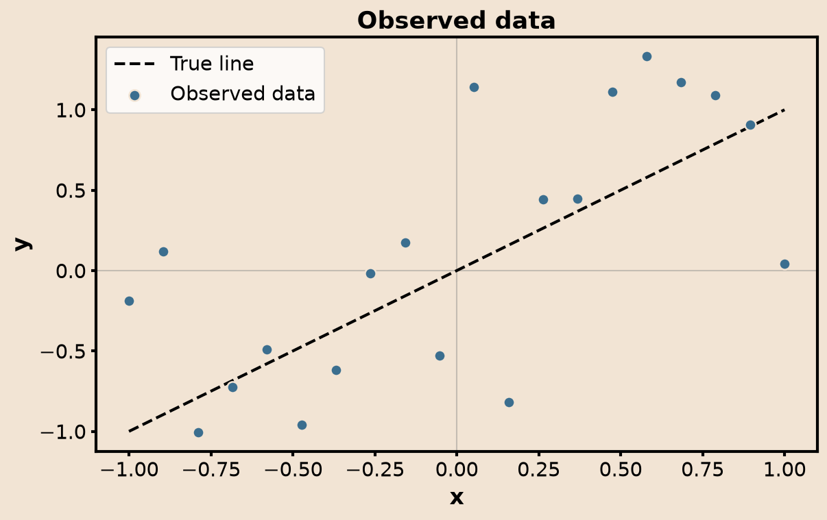
Running the resampling loop times gives us trajectories of the parameter estimate over time:

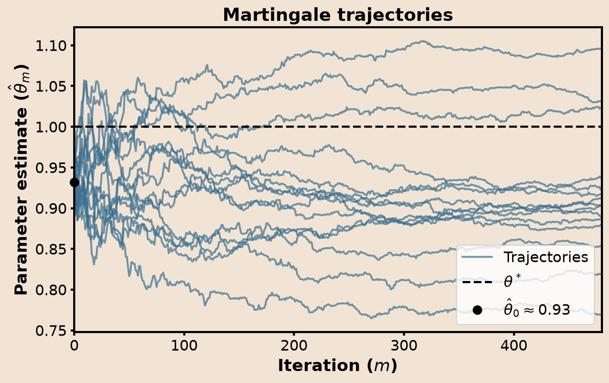
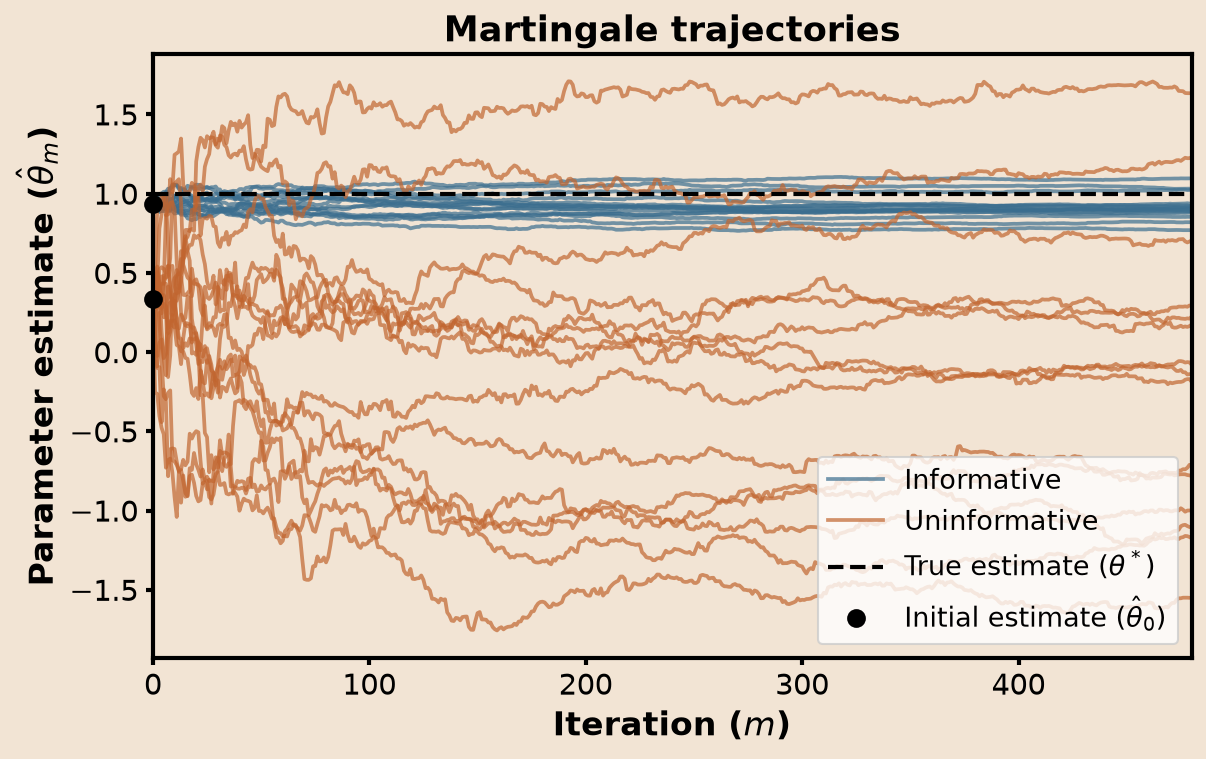
Each trajectory converges to some final value . Collecting all of these gives us the posterior distribution over :

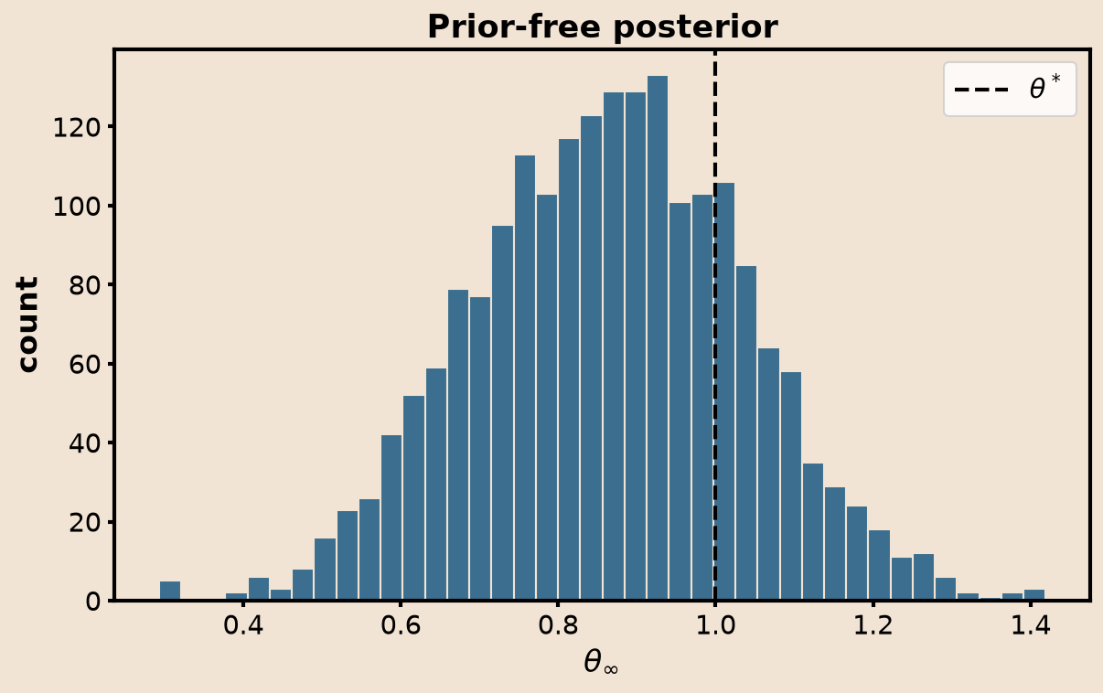
Now we’ll run the procedure on data that’s less informative about the true parameter. By ‘less informative’ I mean the observed ’s are dominated by noise rather than by the true signal . I’ll do this by sampling the query locations from a narrower region, close to zero.

Here’s the data from both runs on the same plot: the informative sample spans , while the uninformative one is squeezed into , so the noise dominates.

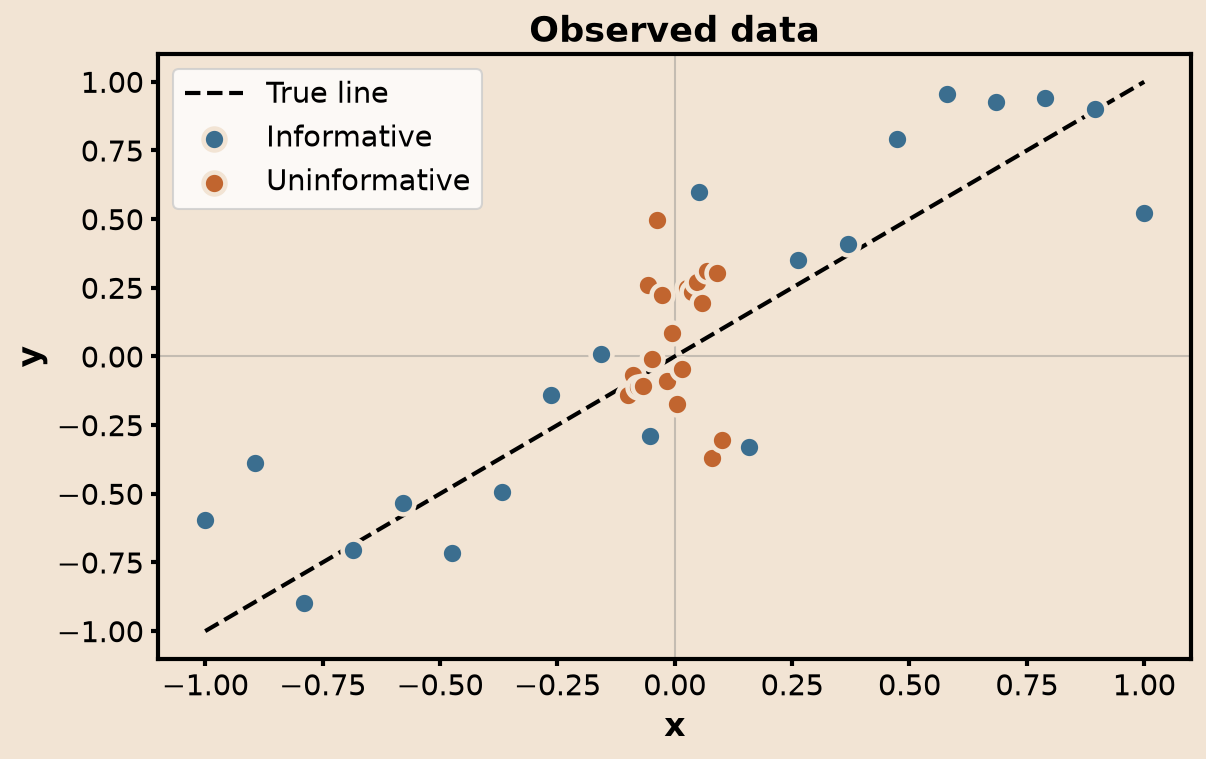
The martingale trajectories tell the same story. The informative run (blue) quickly settles into a tight band around the true , while the uninformative run (orange) wanders much more widely and never really settles down.

And the resulting posteriors make the difference clear: compared to the uninformative case, the informative case has a much tighter distribution that is also closer to the true value.

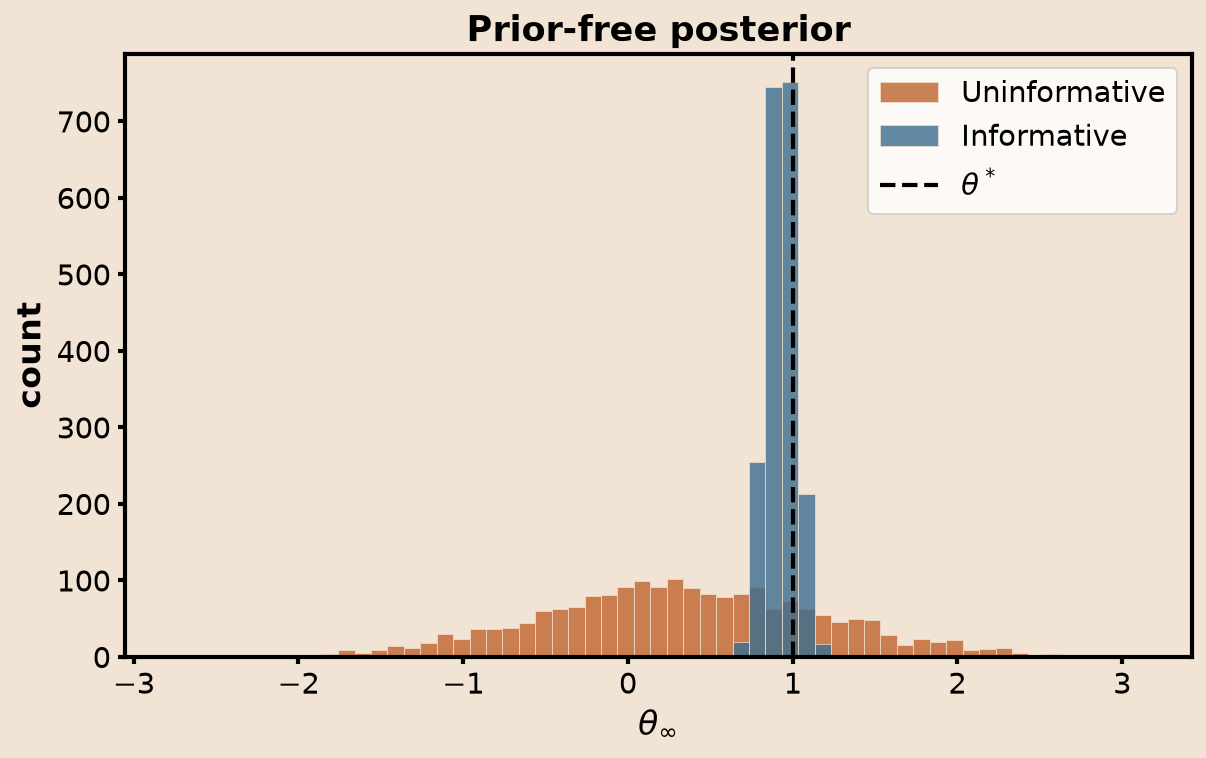
Same procedure, same true model, same noise level. The only thing that changed is how informative the ’s we happened to sample were, and the resulting posterior reflects that difference directly. All without ever needing a prior!

Code for the example above is here.

Acknowledgements §

Thank you to Gerardo for bringing this paper to my attention! Check out his paper where he uses the same martingale-based approach to quantify uncertainty when the model is a neural network.

Post 31/100 §