I derive the vanilla policy gradient and then estimate it with the generalized advantage estimator which can parametrically trade between bias and variance.
Notation:
At time
Policy Gradient
Derivation
Let trajectory
Given a reward function
The finite-horizon undiscounted reward is given by
Now, consider the problem of finding a stochastic policy
which we could solve through gradient ascent:
where
Our next task then is to find an expression for the policy gradient
The probability of a trajectory, conditioned on parameters
where
Evaluating
and may be unknown - Even if they are known, they might be too complex or unknown to differentiate through. 1
To get around this, we can re-write it in terms of easier-to-evaluate log-probabilities.
First we note that
And if we re-arrange, substitute, and simplify:
Plugging back into (2):
And re-writing in terms of an expectation:
Estimation
In practice, we compute
Unfortunately, this is a very high-variance estimate (trust me on this, for now).
In the next section, we introduce a variance reduction technique where we replace
The Generalized Advantage Estimator
In this section, I’ll start by deriving the advantage function.
Then, I’ll show how using this function (instead of the raw reward), provides a lower-variance estimator of
Bias of a baselined policy gradient estimator
A baseline is a function
It turns out that we can introduce any baseline without biasing the policy gradient expectation as long as the baseline does not depend on
Our task is to show that the second term is equal to zero.
First, let
Now let’s look at an expectation for a single timestep
If we substitute
If we re-arrange the integrals over actions, we can express
In this form, it is clear that most of the nested integrals simplify to 1. After collapsing most of the integrals we’re left with
where the underbrace going to zero is a result of applying the log trick shown in the first section (this is also a known property of score functions). Therefore,
implying that expectation of the baselined reward does not depend on
Now that we’ve shown that adding
The advantage function
It turns out that there are several related expressions for the policy gradient (see Schulman et al’s paper for more details). The estimator I derived above used the reward, but there are many other valid expressions all of which have the following form:
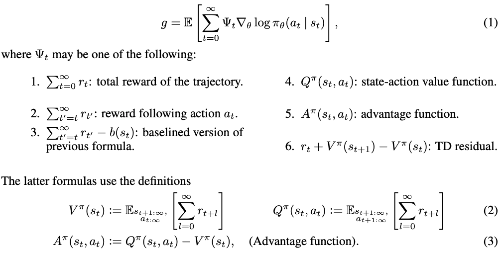
As discussed in Schulman’s paper, it turns out that using the advantage function
Then, the advantage of action
The problem with using the advantage function is that, in practice, it is unknown (we don’t know what the value function is).
One way of approximating the advantage is to use TD residuals.
The TD residual with discount
It turns out that, if
The problem is that if all we have is an approximation of the value function (e.g., a neural network)
If we manipulate it a little, we can re-write this as a discounted sum of two TD differences:
Therefore, we can define a whole family of estimators for the advantage function:
Turns out, that as
Unfortunately, there is no free lunch because our estimator is now in terms of an empirical mean, which unbiased as it may be, is much higher in variance. The empirical mean has high variance because it sums rewards over an entire trajectory, so the randomness from every single action and state transition compounds, causing the final total return to vary significantly from one rollout to the next. In the next section I go into one way of dealing with this.
The generalized advantage estimator
The generalized advantage estimator
This weighted average provides a way of compromising between bias and variance. Consider the following two extremes:
- The 1-step estimator (
): This is . It is stable but biased, as it relies heavily on our approximate value function . - The
-step estimator ( ): This is , the sum of all rewards. It is unbiased but noisy, as the sum of many random rewards has high variance.
In the GAE, the parameter
Thank you for reading! In the next section, I’ll go into how the GAE is used in a popular RL algorithm: PPO.
Resources
Policy gradient
- OpenAI’s Intro to Policy Optimization
- Lilian Weng’s post on policy gradient algorithms
- Daniel Takeshi’s post on policy gradient fundamentals
- Schulman et al.’s original paper on Generalized Advantage Estimation
This is blogpost 13/100
Footnotes
-
Incidentally, differentiating through the transition function
is exactly what I did in this post. The caveat is that I had access to a very nice differentiable simulator. ↩